Using torch.func features

Deepwave supports using torch.func features, such as vmap (vectorising map) and forward-mode automatic differentiation (AD), to perform batch processing and sensitivity analysis. This allows for functional transformations of the wave propagation.

However, there are significant constraints and performance considerations when using these features with Deepwave:

• Property models under vmap: vmap can currently only be applied to property models (e.g., velocity, scattering potential), not to source amplitudes or source/receiver locations. Forward-mode AD is less restricted: the fast-backend jvp of scalar, acoustic and elastic additionally accepts tangents on the source amplitudes and the initial wavefields. Floating-point locations can be differentiated through Hicks interpolation in supported configurations; this is separate from support for batching locations under vmap. See Usage for off-grid locations.

• Backend support: vmap requires the pure-Python backend=”eager” backend (substantially slower than the default C/CUDA backend). Forward-mode AD (`torch.func.jvp` / `torch.autograd.forward_ad`) on the `scalar`, `acoustic` and `elastic` propagators, however, now runs on the fast default C/CUDA backend: internally it routes the tangents through the Born machinery (the Born scattered field is the JVP of the corresponding nonlinear propagator; see Forward-mode AD on the fast backend: scalar_born is the JVP below), so you do not need backend=”eager” for jvp of those three. The propagators with no hand-derived Born-based jvp rule on the compiled backend – scalar_born, acoustic_born, acoustic_vti, viscoacoustic, elastic_born and elastic_vti – do still require backend=”eager” for jvp, and raise an error naming it if you ask for jvp on the default backend. The per-propagator jvp column is in Capability matrix, which is declared in code and checked by conformance probes. With fixed numerical setup, the scalar velocity tangent is linearised through the extension into the PML too; the omitted derivative is the dependence of an inferred max_vel on the model, as explained below.

• max_vel under `vmap`: max_vel has to be given when a model that the maximum wavespeed is computed from is batched by vmap, which hides the concrete values it would otherwise be read from (it fixes the CFL time step and the PML profiles, which are one set of numbers for the whole call in any case). The models the maximum is read from are listed per propagator in Capability matrix; batching any other model does not require it. Under every other transform – grad, jacrev, jvp – the model’s values are readable, so max_vel is inferred exactly as it is outside the transform. One combination needs it whatever is batched: under torch.compile of a vmapped function you must pass max_vel= explicitly, because the readability check is skipped while compiling, so omitting it surfaces PyTorch’s own “.item() on a Tensor … with vmap” error instead of Deepwave’s. Passing it explicitly is still worth doing whenever you want the internal time step pinned across an inversion, transform or no transform.

• Native Batching Preferred: Deepwave already has native support for batched property models. If your goal is simply to propagate a batch of models, the native C/CUDA backend (which handles batch dimensions automatically) will be much faster than using vmap with the eager backend. torch.func is primarily useful for more advanced use cases.

Forward-Mode AD for Scattering (Jacobian-Vector Product)

We can use torch.func.jvp to compute the scattered wavefield (the linearised response) due to a perturbation in the velocity model. This is mathematically equivalent to the Born approximation. In this example, we verify that the output of jvp applied to the nonlinear scalar propagator matches the output of the explicit scalar_born propagator.

First, we define a wrapper for the simulation that fixes the arguments we are not differentiating with respect to. We keep backend=”eager” here because this same wrapper is reused for the vmap composition later (vmap requires the eager backend). For a standalone jvp of scalar you can drop backend=”eager” and run on the fast default backend — see Forward-mode AD on the fast backend: scalar_born is the JVP below:

def forward_sim(v):
    # eager backend so this wrapper can also be used with vmap below,
    # which is also why max_vel is given: vmap hides the velocity values
    # it would otherwise be inferred from.
    return deepwave.scalar(
        v,
        dx,
        dt,
        source_amplitudes=source_amplitudes,
        source_locations=source_locations,
        receiver_locations=receiver_locations,
        pml_freq=freq,
        max_vel=2000,
        backend="eager",
    ).receiver_amplitudes

Then we can calculate the Jacobian-Vector Product. Here v_bg is the background velocity model (the point at which we linearise) and scatter is the perturbation (the direction in which we differentiate):

# Calculate the Jacobian-Vector Product
# primals = (v_bg,), tangents = (scatter,)
_, out_jvp = torch.func.jvp(forward_sim, (v_bg,), (scatter,))

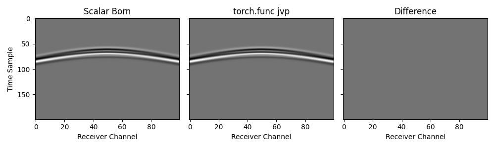
Forward-mode AD on the fast backend: scalar_born is the JVP

scalar_born is the exact discrete forward-mode derivative (JVP) of scalar with respect to the velocity model, and it runs on the fast C/CUDA backend. This is exactly the relationship that torch.func.jvp(scalar, ...) now exploits internally: a standalone jvp of scalar (without vmap) runs on the fast default backend, so backend="eager" is not required. Nor is max_vel: a forward-mode-wrapped model’s values are readable, so the maximum wavespeed is inferred from them exactly as it is without the transform. It is passed below all the same, to pin the internal time step. Define a fast-backend wrapper:

def forward_fast(v):
    return deepwave.scalar(
        v, dx, dt,
        source_amplitudes=source_amplitudes,
        source_locations=source_locations,
        receiver_locations=receiver_locations,
        pml_freq=freq, max_vel=2000,   # no backend="eager"
    ).receiver_amplitudes

Then, for a background model v and a perturbation direction dv:

primal, tangent = torch.func.jvp(forward_fast, (v,), (dv,))   # fast backend

agrees, up to floating-point error, with the following call using the same numerical setup:

out = deepwave.scalar_born(
    v, dx, dt,
    dv=dv,                       # dv is the tangent direction
    source_amplitudes=source_amplitudes,
    source_locations=source_locations,
    sc_receiver_locations=receiver_locations,
    bg_receiver_locations=receiver_locations,
    pml_freq=freq,
    max_vel=2000,
)
bg_receivers = out.bg_receiver_amplitudes
sc_receivers = out.sc_receiver_amplitudes
# sc_receivers == tangent   (the forward-mode/Born scattered field)
# bg_receivers == primal    (the unperturbed scalar field)

on the default (fast) backend. This equivalence holds including when the perturbation overlaps the source cell: scalar pre-scales each source by -v^2 dt^2, so its derivative contributes an extra scattered point source -2 v dv dt^2 f, and scalar_born already injects exactly this term via its second (scattered) source. No separate source argument is needed.

An important qualification is the maximum wave speed. Both the PML profile’s amplitude and the internal time step are built from it, and neither scalar_born nor torch.func.jvp linearises that dependence: the maximum arrives as a Python number, a constant of the call. The Born and JVP paths agree for matching resolved settings even when both omit this dependence; their agreement alone does not check it. To interpret either as the derivative of a call with respect to its model, pin max_vel and the other numerical settings. torch.func.jvp on scalar warns when the velocity tangent is non-zero inside the PML and max_vel was left to be inferred. That warning is conservative: an interior maximum can also move, so absence of the warning does not establish that the inferred bound is constant under the perturbation. The perturbation itself may live anywhere, the outermost cells of the model included: they are extended outwards to fill the absorbing layer and the finite-difference halo, on the scattering model as on the background velocity, so the linearisation is exact there too. This is verified in tests/test_scalar_born.py (test_born_is_jvp_of_scalar, test_born_jvp_model_edge), tests/test_born_edge_linearisation.py and tests/test_scalar_jvp.py.

So: scalar_born and torch.func.jvp(scalar, ...) are two entry points to the same fast-backend linearisation. Use scalar_born directly for the explicit, ergonomic RTM/LSRTM tool, and torch.func.jvp when you want the torch.func transform API itself – for example to differentiate with respect to the source amplitudes or initial wavefields as well as v, or to compose with vmap (below; vmap still requires backend="eager").

Batched Sensitivity Analysis with vmap

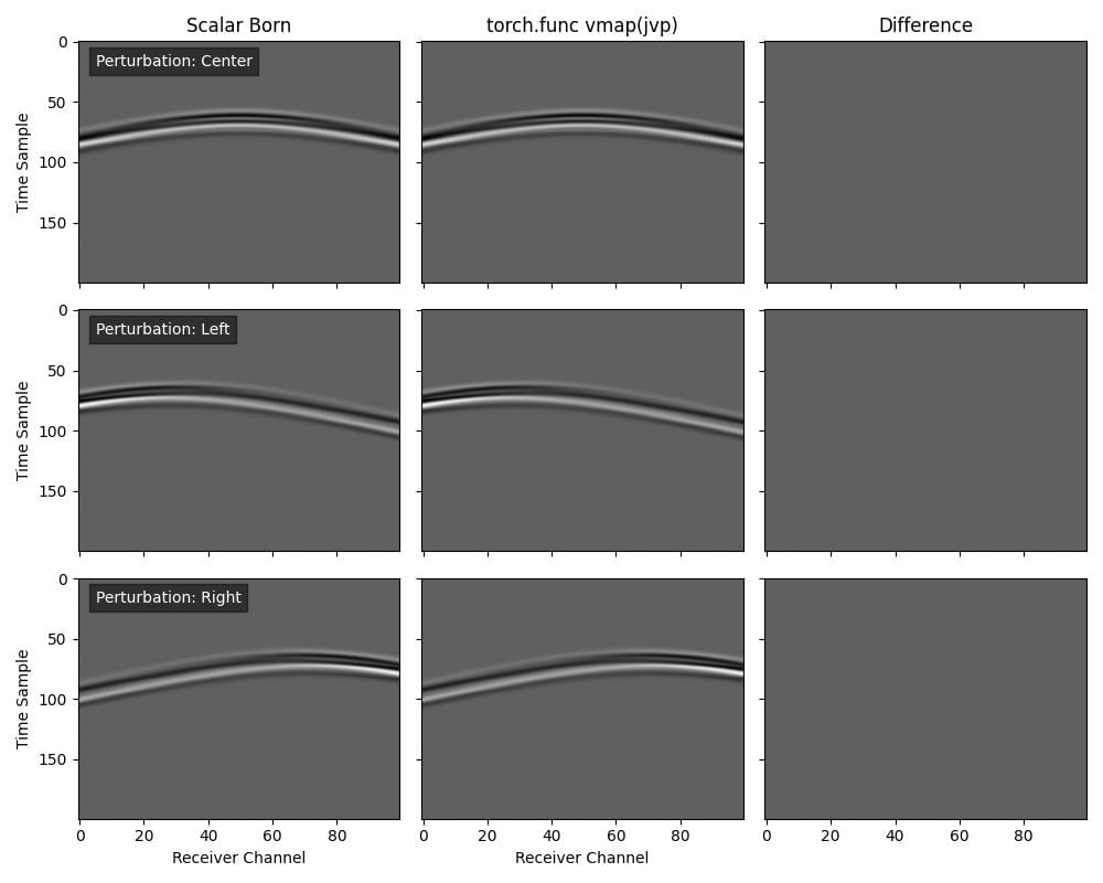
If we want to evaluate the scattering response for a batch of different perturbations (e.g., anomalies at different locations), we can combine vmap with jvp.

We define a function that computes the JVP for a single tangent vector (perturbation), and then use vmap to vectorise it over a batch of perturbations:

# Define a function that takes a single perturbation and returns
# its JVP
def get_jvp(tangent):
    # We fix the primal (v_bg) and vary the tangent
    return torch.func.jvp(forward_sim, (v_bg,), (tangent,))[1]

# Vectorise `get_jvp` over the perturbation input
out_vmap = torch.func.vmap(get_jvp)(scatter_batch)

Reverse-mode transforms (grad, vjp, jacrev, hessian)

torch.func’s reverse-mode transforms – torch.func.grad(), torch.func.vjp(), torch.func.jacrev(), and torch.func.hessian(), which is built from them – require backend="eager" on every propagator that has a compiled backend. There is no fast-backend equivalent of the Born trick that makes jvp work on the compiled backend: these transforms differentiate a tensor that does not carry requires_grad through the forward pass, so the compiled backend’s forward saves nothing for its hand-derived adjoint, and the transform then asks for that adjoint anyway. Deepwave detects this and raises, naming backend="eager":

RuntimeError: deepwave.scalar's backward pass was reached without the
state that its forward pass saves. On Deepwave's compiled (C/CUDA)
backend that happens under the reverse-mode torch.func transforms ...
Re-run the propagator with the pure-PyTorch eager backend,
backend="eager" ...

On a propagator whose compiled backend has no hand-derived second-order rule (scalar_born and viscoacoustic among them) the second-order guard is reached first and reports the same situation in its own words: a reverse-mode transform runs its backward with grad enabled, which is exactly what that guard watches for, so the message names double-backward rather than torch.func. The remedy is the same: backend="eager".

So, with backend="eager":

def loss(v):
    return (
        deepwave.scalar(
            v, dx, dt,
            source_amplitudes=source_amplitudes,
            source_locations=source_locations,
            receiver_locations=receiver_locations,
            pml_freq=freq,
            max_vel=2000,
            backend="eager",
        ).receiver_amplitudes ** 2
    ).sum()

g = torch.func.grad(loss)(v_bg)

None of this affects an ordinary .backward() or torch.autograd.grad(), which are the usual way to get a gradient out of Deepwave and run on the fast backend: reach for the reverse-mode torch.func transforms only when you want the functional API itself (to compose with vmap, say). For Hessian-vector products on the fast backend, use torch.autograd.grad(..., create_graph=True) on scalar, acoustic or elastic – see Hessian and the “Second-order (create_graph)” column of Capability matrix.

Returning a whole PropagatorOutput from a transformed function

The transformed function does not have to reduce to a single tensor. deepwave.PropagatorOutput and deepwave.AuxiliaryState are registered as PyTorch pytree nodes, so a transform sees the tensors inside them: the children of an output are its tuple elements in return order, with the auxiliary state expanding into the tensors it holds, so the leaves are exactly the output’s tensors. That means the whole output can be mapped, carried as an auxiliary value, or compiled:

batched = torch.func.vmap(
    lambda v: deepwave.scalar(
        v, dx, dt,
        source_amplitudes=source_amplitudes,
        source_locations=source_locations,
        receiver_locations=receiver_locations,
        pml_freq=freq, max_vel=2000, backend="eager",
    )
)(torch.stack([v1, v2]))

batched.receiver_amplitudes.shape     # (2, n_shots, n_receivers, nt)

def loss_and_output(v):
    out = deepwave.scalar(v, dx, dt, ..., backend="eager")
    return (out.receiver_amplitudes ** 2).sum(), out

jacobian, out = torch.func.jacrev(loss_and_output, has_aux=True)(v)

The field names and the info of a rebuilt output are the ones of the run that produced it, and its auxiliary_state keeps the recorded run parameters that let a later call check it, so an output that has been through a transform is still usable as initial_state=. vmap still maps property models only, so mapping the source amplitudes is refused with its own message.

Full example code