Reverse-Time Migration (RTM)
Reverse-time migration forms an image of subsurface reflectivity by combining a source wavefield propagated through a background model with receiver data propagated by the adjoint. A common imaging condition sums their zero-lag cross-correlation over time. Coherent arrivals can highlight reflectors, but acquisition geometry, the source wavelet and modelling errors also affect the image.
This example uses the adjoint of the Born operator instead. Define a velocity perturbation dv that starts at zero, compare its modelled scattered data with observations, and differentiate that misfit with respect to dv. The negative gradient is a migration image in this parameterisation. Its correlation includes the derivative of the discrete wave equation: spatial stencil and velocity factors, source scaling, PML terms and model padding. It is not simply the product of the two raw wavefields. See Custom imaging condition for a raw correlation image and illumination compensation, and Forward operators and their derivatives for the derivative.
For a fixed Born map B and loss ||B dv - d||^2 / N, the gradient at dv = 0 is -2 B.T d / N. With a data mute M, as below, it is -2 B.T M.T M d / N. These are discrete adjoint identities under the conditions in What Deepwave guarantees about gradients; compiled model gradients with CFL substepping or a larger sampling interval approximate the time sum. Writing the image as a gradient also lets optimisers and regularisers act on it directly, as Least-Squares Reverse-Time Migration (LSRTM) does over multiple iterations.
Born migration and the first FWI update
With deepwave.scalar_born(), the route this example takes. The Born propagator takes a background velocity model v_mig and a scattering potential dv, and returns the singly-scattered data that dv produces. Start from dv = 0, so the modelled scattered data is zero and the residual is the whole recorded scattered dataset, and take one gradient:
scatter = torch.zeros_like(v_mig, requires_grad=True)
out = scalar_born(
    v_mig, dx, dt,
    dv=scatter,
    source_amplitudes=source_amplitudes,
    source_locations=source_locations,
    sc_receiver_locations=receiver_locations,
    pml_freq=freq,
)
loss = torch.nn.MSELoss()(out.sc_receiver_amplitudes, observed_scatter)
loss.backward()
# scatter.grad is the RTM image (negated: the gradient points away
# from the image, and an optimiser step follows it downhill).
With plain deepwave.scalar(), the gradient with respect to velocity gives the first update direction for FWI. Here dv is a velocity perturbation, so the two routes use the same linearisation when the background, fixed numerical setup, receiver sampling and data weighting match. Their gradients agree only when the residuals also match: for example, when the Born observations are the full observed data minus the background prediction. A mute alone need not achieve this.
Use scalar_born to hold the background fixed and solve a linear least-squares problem for dv. Linearity does not make the inverse problem well-posed: limited aperture and bandwidth can leave poorly constrained or unobservable perturbations. Regularisation and a suitable background remain necessary considerations; see Least-Squares Reverse-Time Migration (LSRTM).
Either way, one call to backward() on one shot gives that shot’s contribution; the rest of this page is about the two practical problems that stand between that and an image of the whole Marmousi model.
Muting the direct arrival
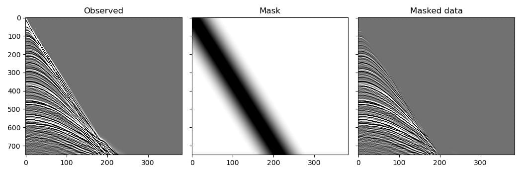
Born modelling produces only singly-scattered waves, but the recorded data also contains the direct arrival, which is far stronger. Trying to explain it with a scattering potential puts a large artefact in the image. Least-Squares Reverse-Time Migration (LSRTM) handles this by modelling the direct arrival and subtracting it; here it is muted instead, with a mask that attenuates the data around the expected direct-arrival time. To avoid introducing high frequencies into the data with a sharp cut-off, we use a tapered mute for the mask:
mask = torch.ones_like(observed_data)
flat_len = 100
taper_len = 200
taper = torch.cos(torch.arange(taper_len)/taper_len * math.pi/2)
mute_len = flat_len + 2*taper_len
mute = torch.zeros(mute_len, device=device)
mute[:taper_len] = taper
mute[-taper_len:] = taper.flip(0)
v_direct = 1700
for shot_idx in range(n_shots):
    sx = (shot_idx * d_source + first_source) * dx
    for receiver_idx in range(n_receivers_per_shot):
        rx = (receiver_idx * d_receiver + first_receiver) * dx
        dist = abs(sx - rx)
        arrival_time = dist / v_direct / dt
        mute_start = int(arrival_time) - mute_len//2
        mute_end = mute_start + mute_len
        if (mute_start > nt):
            continue
        actual_mute_start = max(mute_start, 0)
        actual_mute_end = min(mute_end, nt)
        mask[shot_idx, receiver_idx,
             actual_mute_start:actual_mute_end] = \
            mute[actual_mute_start-mute_start:
                 actual_mute_end-mute_start]
observed_scatter_masked = observed_data * mask
Fitting the whole survey in memory
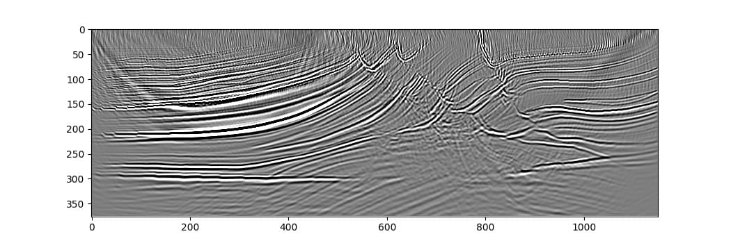
This example migrates the entire Marmousi model and dataset – 115 shots – which would probably not fit in memory if every shot were propagated simultaneously, as the smaller examples do. Instead we propagate batches of shots and accumulate the gradients over all the batches before taking a step with the optimiser. Each time we backpropagate, PyTorch adds to the existing gradient values. We zero the gradients before this loop and weight each batch’s mean loss by its fraction of the total shot count. With the same number of receivers and samples per shot, this gives the full-survey mean loss and gradient, within floating-point rounding. Simply summing batch means would overweight a smaller final batch and change the update scale when the batch size changes. We tell the optimiser to use this gradient to take a step only after the loop over shot batches has completed, so using batches changes neither the update nor the final result. A PyTorch data loader could equally have been used to split the data into batches, with equivalent results:
# Create scattering amplitude that we will invert for
scatter = torch.zeros_like(v_mig)
scatter.requires_grad_()

# Setup optimiser to perform inversion
optimiser = torch.optim.SGD([scatter], lr=1e9)
loss_fn = torch.nn.MSELoss()

# Run optimisation/inversion
n_epochs = 1
n_batch = 46  # The number of batches to use
n_shots_per_batch = (n_shots + n_batch - 1) // n_batch
for epoch in range(n_epochs):
    epoch_loss = 0
    optimiser.zero_grad()
    for batch in range(n_batch):
        batch_start = batch * n_shots_per_batch
        batch_end = min(batch_start + n_shots_per_batch,
                        n_shots)
        if batch_end <= batch_start:
            continue
        s = slice(batch_start, batch_end)
        out = scalar_born(
            v_mig, dx, dt,
            dv=scatter,
            source_amplitudes=source_amplitudes[s],
            source_locations=source_locations[s],
            sc_receiver_locations=receiver_locations[s],
            pml_freq=freq
        )
        loss = (
            loss_fn(out.sc_receiver_amplitudes * mask[s],
                    observed_scatter_masked[s])
        ) * (batch_end - batch_start) / n_shots
        epoch_loss += loss.item()
        loss.backward()
    print(epoch_loss)
    optimiser.step()
Note that n_epochs is 1: this is migration, not inversion. The single optimiser step turns the accumulated gradient into the image. Because the scattering potential starts at zero and the learning rate is a constant, the image is the negative gradient times the learning rate. Its amplitude depends on that choice, the loss normalisation, source calibration and illumination; it is not a calibrated velocity perturbation. Running more iterations turns it into LSRTM, which corrects for uneven illumination and the source wavelet, but which also needs a more careful setup to converge to something useful.
Batching with this loss weighting gives the full-survey update within floating-point rounding. For an inversion that runs for many iterations it might converge faster to instead take a step after every batch, or after every small number of batches, using randomly selected shots in each batch. This is the way training is typically done for neural networks, and is easy to set up here too: as simple as moving optimiser.zero_grad() and optimiser.step() inside the loop over batches in the code above.
Running this example
It needs the Marmousi files, marmousi_vp.bin and marmousi_data.bin, in the directory it is run from; python docs/get_marmousi.py produces both (see Examples). Running it with DEEPWAVE_SMOKE=1 set needs no download: it migrates a small generated stand-in model instead, which checks that the code runs but produces nothing worth looking at. If you want a migration you can run immediately and interpret, the one-file FWI example is the closest self-contained relative – its first iteration’s gradient is a velocity image, with the residual and numerical qualifications described above.
Where to go next
Least-Squares Reverse-Time Migration (LSRTM) – iterating instead of taking a single step.
Custom imaging condition – replacing the zero-lag cross-correlation, and illumination compensation.
Joint Migration Inversion – solving for the background velocity and the reflectivity together.
Born Modelling with the Scalar Wave Equation – what the Born propagator computes, precisely.