Forward modelling with Marmousi velocity model
This example loads the Marmousi 1 \(v_p\) (P-wave velocity) model, specifies source and receiver locations, and uses Deepwave to perform forward modelling: propagating the sources through the model to generate synthetic receiver data. It is a good starting point if you have completed Quick Start and want to see the scalar propagator used on a realistic model.
First, we need to import the necessary packages:
import torch
import matplotlib.pyplot as plt
import deepwave
from deepwave import scalar
We then choose which device we wish to run on, specify the size of the model, and load it:
from get_marmousi import load_vp

device = torch.device('cuda' if torch.cuda.is_available()
                      else 'cpu')
ny = 751
nx = 2301
dx = 4.0
v = load_vp().to(device)
load_vp is in docs/get_marmousi.py, the script described below. It reads marmousi_vp.bin from the current directory and checks that it is in the layout Deepwave 0.1.0 writes, so that every Marmousi example fails in the same recognisable way when the file is missing or stale rather than each rolling its own torch.from_file() call.
Dimension 0 is depth and dimension 1 is horizontal position, the convention this documentation uses throughout (see Dimension order and the axis convention).
The file that marmousi_vp.bin above needs to exist for this to work, plus marmousi_data.bin used by the later Marmousi examples (RTM, LSRTM, FWI, joint migration inversion, custom imaging condition, and the two fuller distributed-execution examples), are not shipped with Deepwave. This is not an oversight: the original Marmousi model was created by the Institut Francais du Petrole (IFP) and has been distributed academically for decades (including from the Geoazur WIND project, its most commonly cited current home) without IFP ever publishing redistribution terms for it – unlike its later elastic descendant, Marmousi2/AGL Elastic Marmousi, which is a different, larger dataset explicitly released by SEG’s open-data initiative under CC BY 4.0. Because that permission has not been confirmed for the model these examples use, Deepwave does not host or redistribute a copy itself; instead, get it directly from the original source and let Deepwave generate the synthetic data locally:
python docs/get_marmousi.py
Run this once, from whichever directory you will run the Marmousi examples from (that is where it writes its output, and where load_vp above looks for it). It downloads the Marmousi 1 \(v_p\) model from the Geoazur WIND project above, verifies it against a recorded SHA-256 checksum, transposes it into the 751 x 2301 depth-first little-endian float32 layout this page’s code expects and writes that out as marmousi_vp.bin, then runs this very example’s forward-modelling recipe at full size to generate marmousi_data.bin. Generating the full 115-shot dataset can take a while on CPU; pass --smoke for a small, fast version of both files if you just want to try the pipeline out. If you downloaded marmousi_vp.bin before Deepwave 0.1.0, it is in the older untransposed layout and must be regenerated: the examples detect this and tell you so rather than silently propagating through a rotated model. See docs/get_marmousi.py’s own docstring for the full details, including the citation to give the model in any resulting publication: Bourgeois et al. (1991), “Marmousi, model and data”.
If you only want to check that this example runs, setting DEEPWAVE_SMOKE=1 (see Running the examples) replaces the downloaded model with a generated stand-in of the same shape and velocity range, so no download is needed. The stand-in is not Marmousi, and nothing in the resulting figures is worth interpreting.
Next we specify where to place the sources and receivers, and what the source wavelets should be. Deepwave can propagate batches of shots simultaneously to improve computational performance; the shots do not interact with each other, and the results are identical to propagating them individually. Shots propagated together are assumed to have the same number of sources and receivers, with locations given as Tensors of shape [shot, source, space] and [shot, receiver, space] respectively, and source amplitudes as a Tensor of shape [shot, source, time]. Many applications use only one source per shot, so the source dimension is often of unit length, but Deepwave supports multiple sources per shot:
n_shots = 115

n_sources_per_shot = 1
d_source = 20  # 20 * 4m = 80m
first_source = 10  # 10 * 4m = 40m
source_depth = 2  # 2 * 4m = 8m

n_receivers_per_shot = 384
d_receiver = 6  # 6 * 4m = 24m
first_receiver = 0  # 0 * 4m = 0m
receiver_depth = 2  # 2 * 4m = 8m

freq = 25
nt = 750
dt = 0.004
peak_time = 1.5 / freq

# source_locations
source_locations = torch.zeros(n_shots, n_sources_per_shot, 2,
                               dtype=torch.long, device=device)
source_locations[..., 0] = source_depth
source_locations[:, 0, 1] = (torch.arange(n_shots) * d_source +
                             first_source)

# receiver_locations
receiver_locations = torch.zeros(n_shots, n_receivers_per_shot, 2,
                                 dtype=torch.long, device=device)
receiver_locations[..., 0] = receiver_depth
receiver_locations[:, :, 1] = (
    (torch.arange(n_receivers_per_shot) * d_receiver +
     first_receiver)
    .repeat(n_shots, 1)
)

# source_amplitudes
source_amplitudes = (
    deepwave.wavelets.ricker(freq, nt, dt, peak_time)
    .repeat(n_shots, n_sources_per_shot, 1)
    .to(device)
)
Like the rest of this documentation, this example uses dimension 0 as depth and dimension 1 as horizontal position, with the source and receiver locations matching that choice. That is a documentation convention, not a requirement: Deepwave attaches no physical meaning to any axis and treats both spatial dimensions equally, so the model and its locations could equally have been transposed. See Dimension order and the axis convention.
That is all the setup forward modelling needs, so we are ready to call Deepwave. To keep the results as accurate as possible, we specify 8th order accurate spatial finite differences:
out = scalar(v, dx, dt, source_amplitudes=source_amplitudes,
             source_locations=source_locations,
             receiver_locations=receiver_locations,
             accuracy=8,
             pml_freq=freq)
The pml_freq parameter is optional: if you omit it, Deepwave infers it from the peak of the source amplitudes’ spectrum, which for the Ricker wavelet above is the freq we built it with. Passing it, as here, is still recommended for anything you publish, since an inferred value makes the absorbing boundary depend on the wavelet (see Choosing pml_freq). You can see that the source and receiver Tensors that we provided were also optional. You can instead (or in addition) provide initial wavefields for Deepwave to propagate.
Note that source_depth and receiver_depth above (2 cells, 8 m) place the sources and receivers inside the physical model, close to its top edge. The default 20-cell PML is padding outside that model. Its material values are extended from the model’s edge cells, so differentiation through that extension adds contributions to the velocity gradient at those cells (see Large gradients at edges). See Boundary conditions for the full explanation of what the PML does, and for when you might instead want a source/receiver-free absorbing margin or a reflective (rigid/free) edge.
The number of time steps to propagate for (and thus the length of the output receiver data) is specified by the length of the source amplitude. If you are propagating without a source term, then you can instead specify it using the nt keyword parameter.
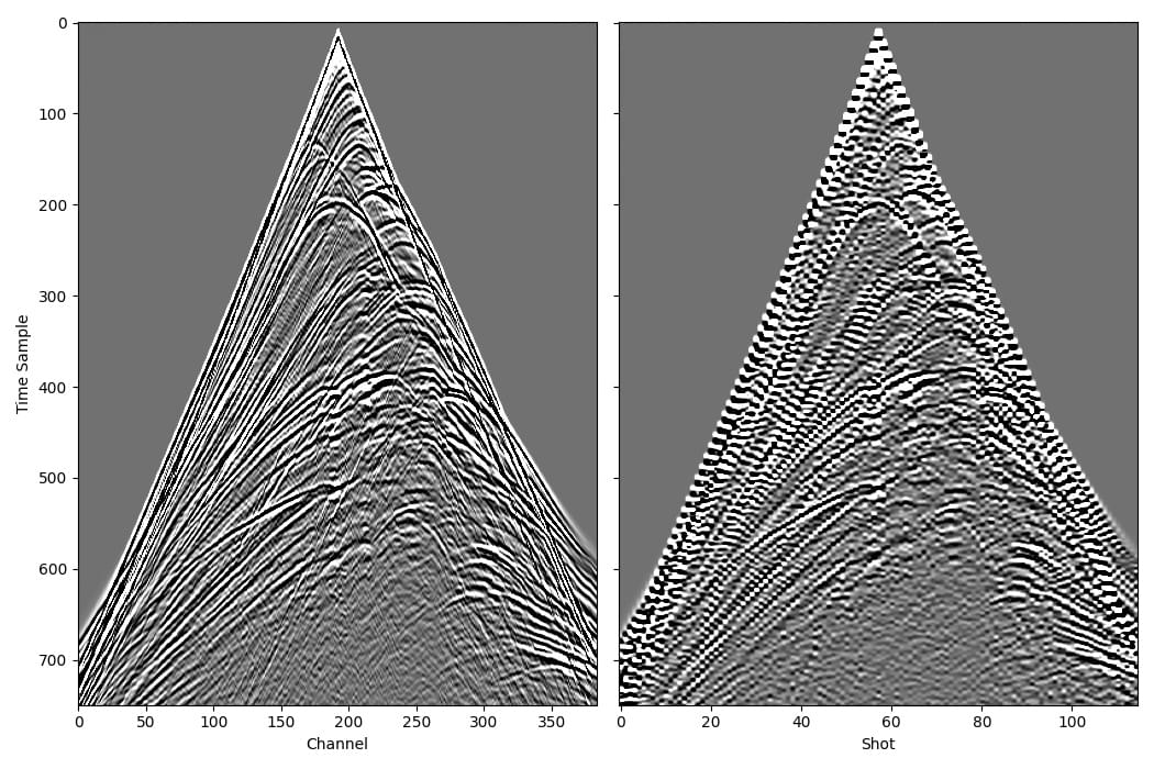
Finally, we will plot one common shot gather and one common receiver gather of the generated data, and then save the data to disk for use in later examples:
receiver_amplitudes = out.receiver_amplitudes
vmin, vmax = torch.quantile(receiver_amplitudes[0],
                            torch.tensor([0.05, 0.95]).to(device))
_, ax = plt.subplots(1, 2, figsize=(10.5, 7), sharey=True)
ax[0].imshow(receiver_amplitudes[57].cpu().T, aspect='auto',
             cmap='gray', vmin=vmin, vmax=vmax)
ax[1].imshow(receiver_amplitudes[:, 192].cpu().T, aspect='auto',
             cmap='gray', vmin=vmin, vmax=vmax)
ax[0].set_xlabel("Channel")
ax[0].set_ylabel("Time Sample")
ax[1].set_xlabel("Shot")
plt.tight_layout()

receiver_amplitudes.cpu().numpy().tofile('marmousi_data.bin')
This example did not need them, but if the output receiver amplitudes contain undesirable wraparound artefacts (where high amplitudes at the end of a trace cause artefacts at the beginning of the trace), the Deepwave propagator options freq_taper_frac and time_pad_frac should help. See Usage for more on them.