Custom imaging condition
This example demonstrates how to use callbacks to implement a custom imaging condition. In seismic imaging, the “imaging condition” is the operation that combines the forward-propagating source wavefield and the backward-propagating receiver wavefield to produce an image of the subsurface. In Full Waveform Inversion (FWI), this image is the gradient of the objective function. The standard imaging condition is a cross-correlation of the two wavefields. This can result in a gradient that is much stronger in areas of high illumination (e.g. near the sources) than in poorly illuminated areas (e.g. deeper in the model or in shadow zones).
To counteract this, we can apply “illumination compensation”, where the gradient is divided by an “illumination map”. This map estimates the amount of source energy that reaches each point in the model. Dividing the gradient by this map boosts the gradient in poorly illuminated regions, which can help the inversion to converge more quickly and produce a more accurate final model.
We will implement a simple source-side illumination compensation using callbacks. First, we calculate the standard gradient for comparison. Then, we define two callback functions to calculate and apply the illumination compensation. The forward_callback is used to create the illumination map by summing the squared wavefield over time and shots. The backward_callback is then used to divide the gradient by this map at the end of the backpropagation step. A small value is added to the illumination map before division to ensure stability.
# Calculate the gradient with illumination compensation
illumination = None

def forward_callback(state):
    global illumination
    if illumination is None:
        illumination = (state.get_wavefield("wavefield_0", view="full").detach()**2).sum(dim=0)
    else:
        illumination += (state.get_wavefield("wavefield_0", view="full").detach()**2).sum(dim=0)


def backward_callback(state):
    if state.step == 0:
        gradient = state.get_gradient("v", view="full")
        gradient /= (illumination + 1e-3 * illumination.max())


out = deepwave.scalar(
    v,
    dx,
    dt,
    source_amplitudes=source_amplitudes,
    source_locations=source_locations,
    receiver_locations=receiver_locations,
    forward_callback=forward_callback,
    backward_callback=backward_callback,
    callback_frequency=1,
)
torch.nn.MSELoss()(out[-1], out_true[-1]).backward()
The forward_callback is called at each time step of the forward propagation. It gets the wavefield for the current time step (which includes all shots) and adds its squared value to the illumination tensor. At the end of the forward pass, illumination will contain the illumination map. The backward_callback is called during backpropagation. We only want it to act at the end, when the full gradient has been computed, so we check if state.step == 0. It then gets a reference to the gradient tensor and divides it in-place by the illumination map. We use view=”full” to ensure we get the tensors for the whole model, including the PML regions.
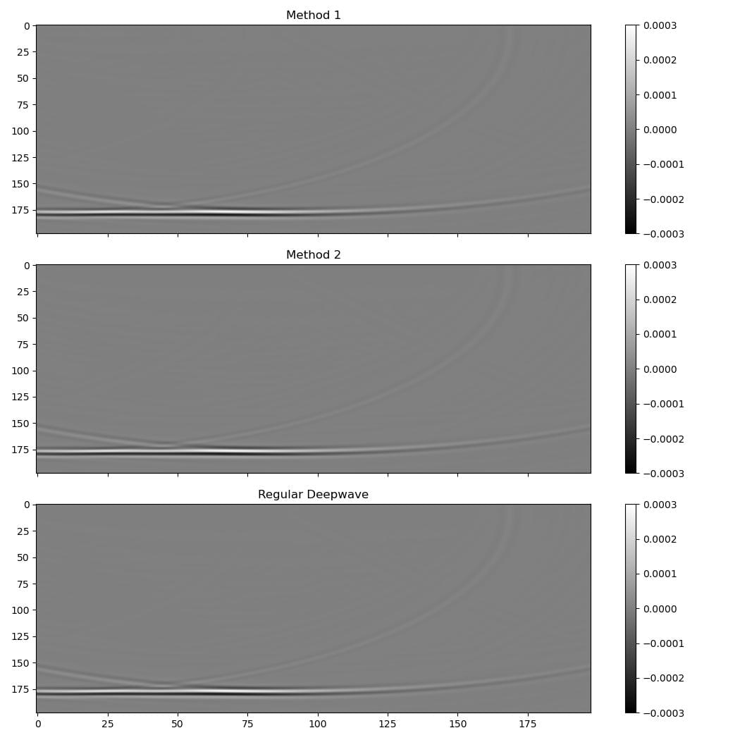
The image below compares the standard gradient (left) with the illumination-compensated gradient (right). The compensated gradient is more balanced and has greater amplitude at depth compared to the standard gradient, which could lead to better FWI results.