Visualising wavefields and gradients with callbacks

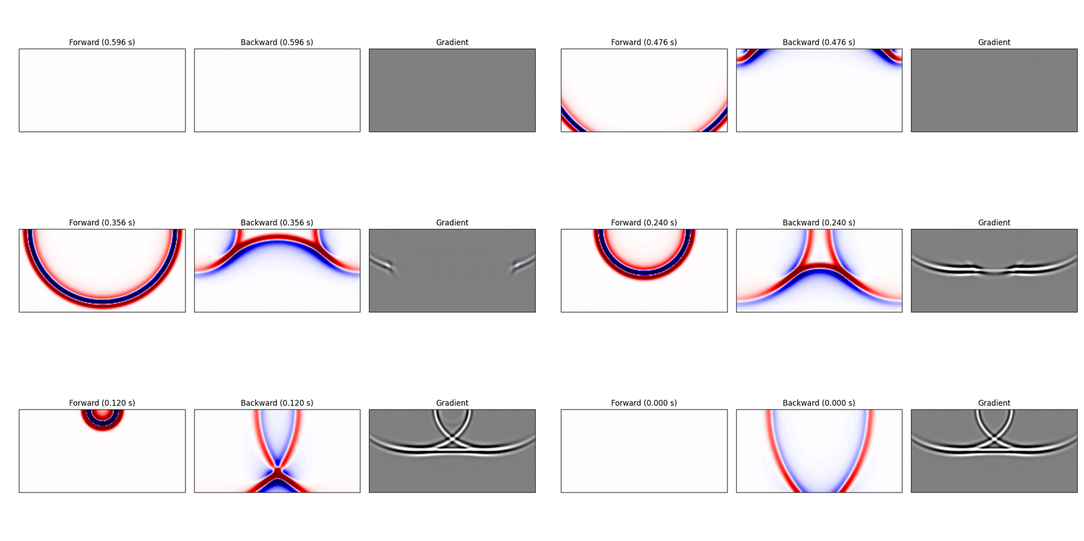
This example demonstrates how to use the callback feature to visualise the wavefields and gradients during forward and backward propagation. Callbacks allow you to execute arbitrary Python code at specified intervals during a simulation, giving you access to the wavefields, models, and gradients.

In this example, we will create an animation that shows three things side-by-side:

1. The forward-propagating wavefield.

2. The backward-propagating wavefield (the adjoint wavefield).

3. The formation of the model gradient during backpropagation.

We setup the propagation as normal, using a simple single layer model. Next, we define two callback functions to store the forward and backward wavefields and the current value of the gradient with respect to the velocity model as backpropagation progresses. We can use regular Python functions for these, but, to show you how it is done, I will use a callable class for the forward callback. The ForwardCallback instance will be called during the forward pass, and the backward_callback function will be called during the backward pass. Each receives a CallbackState object when it is called that provides access to the simulation data. We use these to save the relevant tensors to our snapshot storage. The wavefield names are the same as those in the propagator signature, so the current wavefield is wavefield_0:

# Storage for snapshots from callbacks
callback_frequency = 1
forward_snapshots = torch.zeros(nt // callback_frequency, ny, nx)
backward_snapshots = torch.zeros(nt // callback_frequency, ny, nx)
gradient_snapshots = torch.zeros(nt // callback_frequency, ny, nx)

# Define callback functions

# A callable class, just to show how it is done
class ForwardCallback:
    def __init__(self):
        self.step = 0  # Forward propagation starts at time step 0

    def __call__(self, state):
        """A function called during the forward pass."""
        # We only need the wavefield for the first shot in the batch
        forward_snapshots[self.step] = (
            state.get_wavefield("wavefield_0")[0].cpu().clone()
        )
        self.step += 1

# Could instead have used a function
# def forward_callback(state):
#     forward_snapshots[state.step] = (
#         state.get_wavefield("wavefield_0")[0].cpu().clone()
#     )


def backward_callback(state):
    """A function called during the backward pass."""
    # We use [0] to select the first shot in the batch
    backward_snapshots[state.step] = (
        state.get_wavefield("wavefield_0")[0].cpu().clone()
    )
    gradient_snapshots[state.step] = state.get_gradient("v")[0].cpu().clone()

We then run the simulation, passing our callbacks to the propagator. We set callback_frequency=1 to capture snapshots every time step:

out = deepwave.scalar(
    v,
    dx,
    dt,
    source_amplitudes=source_amplitudes,
    source_locations=source_locations,
    receiver_locations=receiver_locations,
    max_vel=v_true.max().item(),
    forward_callback=ForwardCallback(),
    backward_callback=backward_callback,
    callback_frequency=callback_frequency,
)

torch.nn.MSELoss()(out[-1], out_true[-1]).backward()

Finally, we use Matplotlib to create and save the animation. We iterate through the snapshots backwards in time to see the accumulation of the gradient.

Full example code